Deepmind AI Research Foundations Part 2

Notes I took whilst studying "Google DeepMind: AI Research Foundations". Covers designing and training neural networks as well as the transformer architecture.

Design and Train Neural Networks

• Signal - the underlying pattern we want a model to learn. The information which generalizes to new situations.

• Noise - coincidental patterns/artifacts that don't represent a general rule.

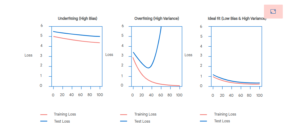
Generalization

A model's ability to generalize to unseen data. There is a balance between bias and variance.

Bias

Underfitting. Ignores the signal. Performs badly on the training and out of sample data.

Can also be due to too few parameters or the model can't capture complex relationships.

Variance

Overfitting. High variance models pay too much attention to the noise, it doesn't learn the general signal but tunes into the coincidental noise.

Performs well in sample but badly out of sample.

Multilayer Perceptron

Input layer, multiple hidden layers and a single output layer. A type of neural network model. Used for classification and regression.

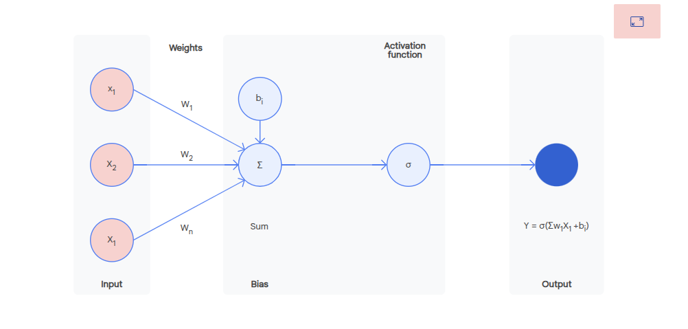
Each neuron has:

1. Inputs - numerical values recieved
2. Weights - inputs have a weight, a vector, a value for each input. These weights are adjusted during training.
3. Bias - allows the neuron to shift it's output up or down independently of the input data
4. Weighted sum - the weight vector x the vector of inputs
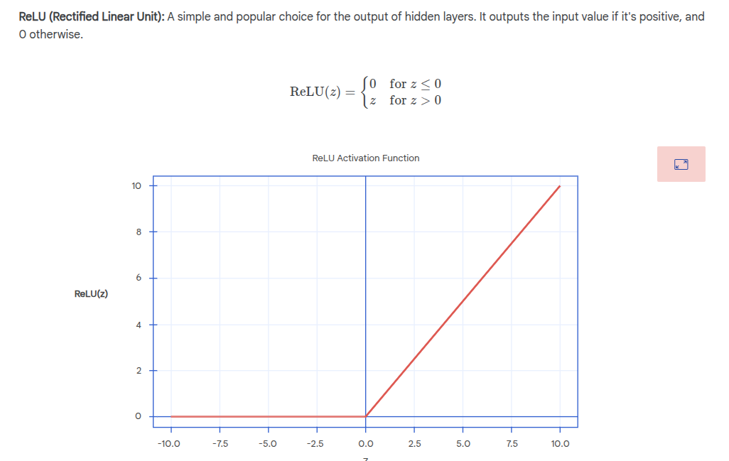
5. Activation function - weighted sum is passed through an activation function to produce the final output. This can be used to introduce non-linearity.

ReLU

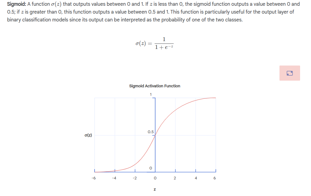
Sigmoid

Used for 2 class problems:

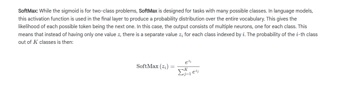
SoftMax

Used for multi class problems. Used to produce a probability distro over many possible outputs.

Here's a single neuron:

Input Layer

Recieves raw data for the task.

Hidden Layers

Layers stacked between input and output layers. Called hidden as the neuron activation values are not directly observable as inputs or outputs. Each subsequent layer builds on the previous one, identifying increasingly abstract and sophisticated patterns.

Output Layer

Produces final prediction as an output.

MLP Comparison

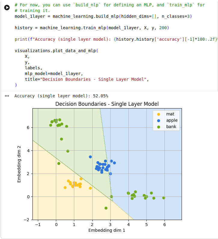
No hidden layers

Here we don't use any hidden layers:

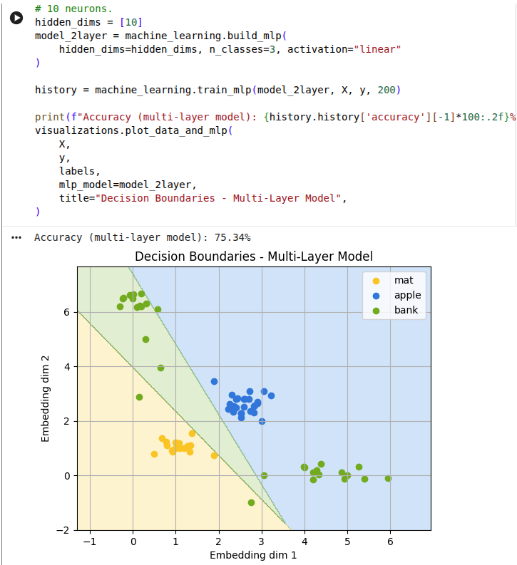
Single hidden layer

Next, we add 10 hidden neurons in a single layer:

Single hidden layer with ReLU

Now we use a non-linear activation function:

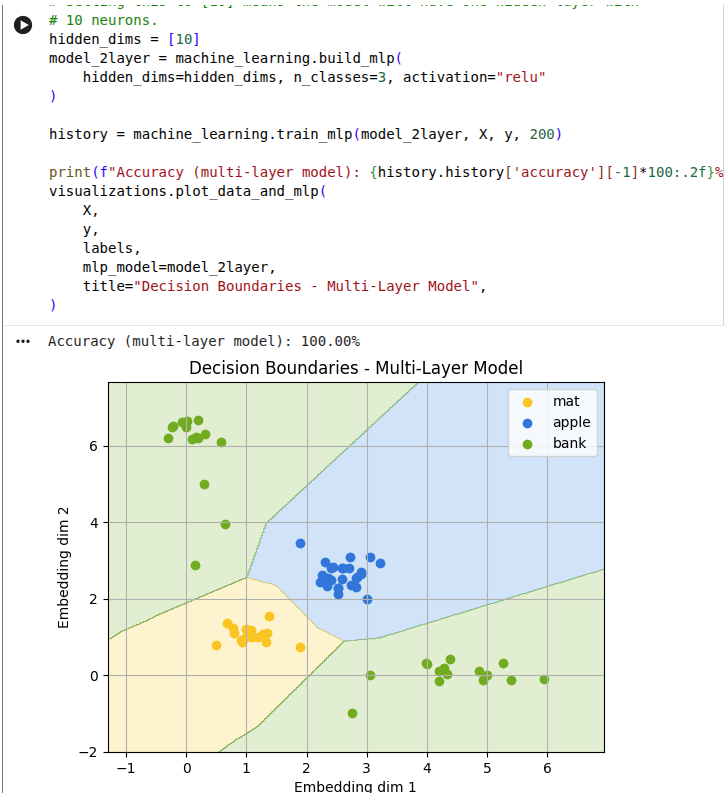
Any multi-layer neural network without a non-linear activation function can also be expressed as a single-layer neural network. Therefore a network without the activation function cannot learn more complex functions that a single-layer MLP.

The key insight is that the first layer learns simple lines, and subsequent layers combine these simple decisions to construct more complex, curved boundaries that are needed to learn from complex data.

Techniques to Mitigate Overfitting

Capacity Control

Reduce the models capacity - the number of layers and number of neurons. It won't have the resources to learn the noise.

Regularization

Weight decay - make the model learn simpler weights by adding a penalty term to the loss function based on the size of its weights. Penalize large weights. Results in smoother and less complex functions.

Dropout

Randomly drop some neurons during training - make the output of those neurons 0. Data looks different at each iteration, forcing the network to learn more robust features. Prevents complex co-adaption between neurons (one neuron relies specifically on another neuron). Make the model learn more independent and useful parameters.

Checkpointing

Saving params at different times during training. Can be used with an early stopping condition.

Early stopping

Stop training once performance on the validation dataset stops improving. If validation error doesn't improve for a number of epochs (the patience) then stop training.

Evaluating Model and System for Safety

From Google AI for Developers:

• Development evaluations - assess model performance during training against launch criteria using adversarial queries and benchmarks.

• Assurance evaluations - independent governance testing for safety policies and dangerous capabilities.

• Red teaming - adversarial testing by specialists to discover weaknesses and improve mitigations.

• External evaluations - independent expert testing to identify limitations and stress-test the model.

Anticipation and Alignment

Anticipation in responsible innovation is not just about
foreseeing technical failures, it is about recognising that
AI systems will interact with complex social, cultural,
organisational, and environmental contexts. This means
being sensitive to uncertainty, exploring a range of
possible outcomes, and considering how technologies may
affect people's lives in ways that go beyond technical
problem solving.

Gradients

• Essential for training neural networks
• Enable automatic learning by updating weights
• Show how to adjust weights to reduce loss
• Point in the direction and magnitude for weight updates
• Larger updates occur when predictions are far from true values
• Smaller updates occur when predictions are close to true values
• Help the model improve predictions over time

Backpropagation

1. Initialization

• Start with randomly initialized weights and biases

2. Forward Pass

• Compute output of each layer sequentially from input to output
• Save layer outputs for use in backward pass

3. Compute Loss

• Calculate loss using the loss function

4. Backward Pass

• Calculate error for the output layer
• Propagate error backward through each layer to compute gradients
• Continue until reaching the input layer

5. Update Parameters

• Adjust weights and biases using gradient descent
• Use stochastic gradient descent (SGD) - update using small random mini-batches instead of full dataset
• Mini-batch gradients are noisy but faster and statistically representative

6. Repeat

• Repeat steps 2-5 for multiple iterations until performance is satisfactory

Binary cross entropy loss:

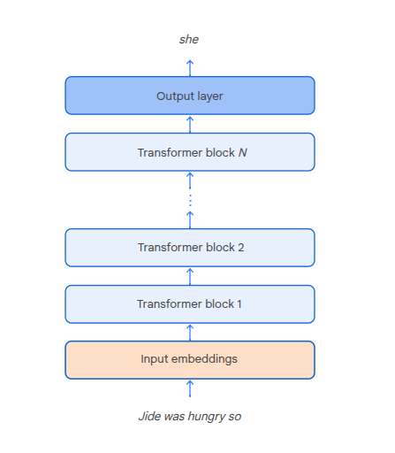
Transformer Architecture

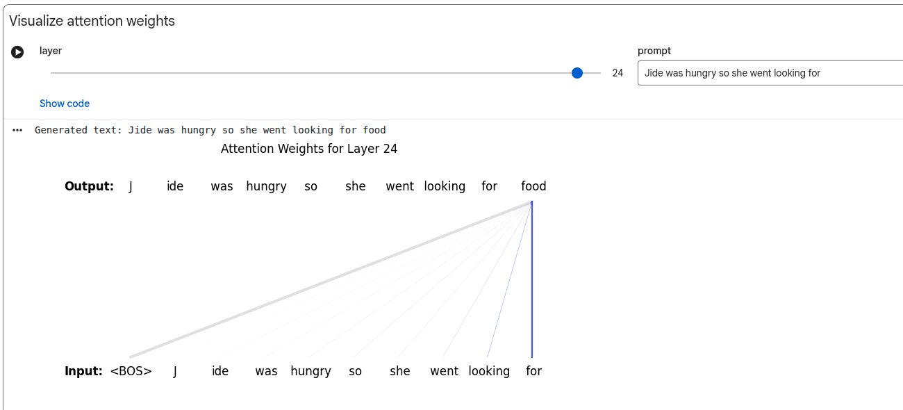
Transformers rely on the attention mechanism to build contextual embeddings from all the tokens in the prompt. They allow for different weight to be applied to the info from each token.

The model "attends" to tokens in a variable way, according to the weight.

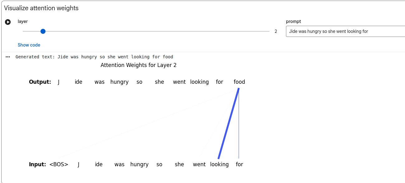
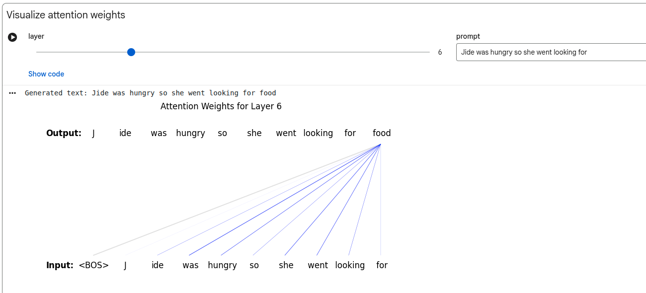
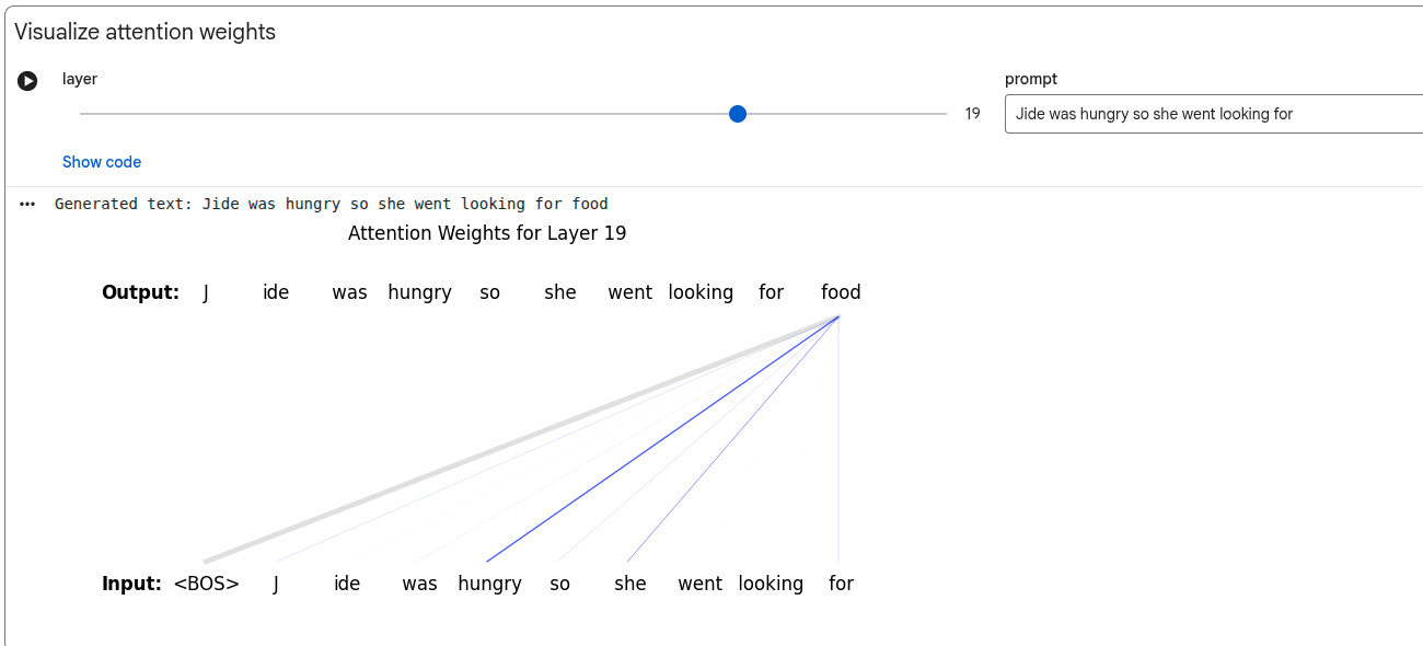
Transformer models have multiple layers - the attention mechanism can operate on every layer.

Attention mechanisms in different layers allow the model to focus on different dependencies between tokens in those layers. Some layers use information across sentences.

Before 2014, attention mechanisms were typically based on position rather than content. Transformers have attention weights which are order invariant - the input is considered unordered from the point of view of the attention mechanism (this is why we need to use attention masking). This means that the output of the attention mechanism is always the same, independent of the order of the previous tokens.

Attention handles long range dependencies much better than RNNs. RNNs are also computationally linear, so can't be parallelized using a GPU.

Parallelism allows you more practically to attend from any word to all other words.

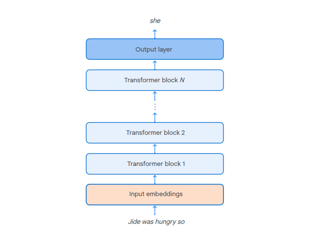
Model Components

• Input embeddings - the token embeddings

• Transformer blocks - stackable blocks like neural net perceptrons. Chain output from one to the input of the next.

• Ouput layer - the last layer, uses a soft-max activation function to give the probability distro over the next token

Contextual Hidden Representations

Transformers incrementally build contextual hidden representations. These are embeddings which combine info from the current token with previous ones.

Each transformer block does this repeatedly, aggregating info from the previous block's contextual hidden representation.

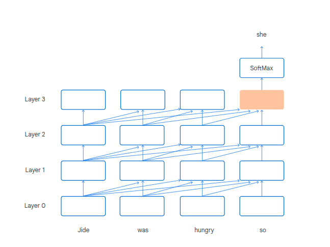
The aggregation is a weighted sum of the contextual represenation of all previous tokens. The weights for the sum are called attention weights.

Computing Contextual Embeddings

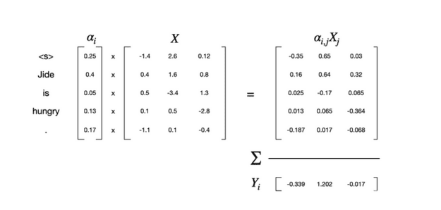
In the above picture, the X array is the embeddings for the token - the embeddings have 3 dimensions and there are 5 tokens.

The alpha vector is the attention weight.

Attention Head

Attention heads compute the attention weights. They are a component of a neural network.

Transformers use content-based dot product self attention.

Tokens can play 3 roles in the computation of attention weights.

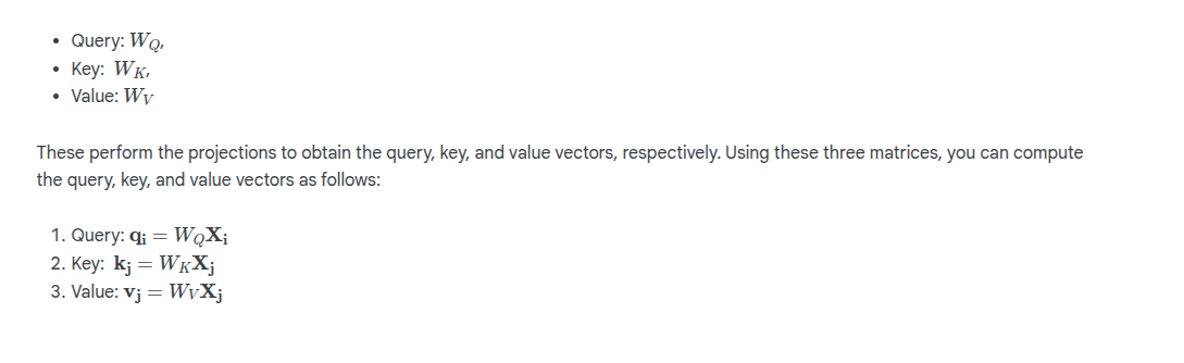
The Query

The current token that is actively seeking information, the one for which we want to calculate a contextual embedding for.

What other tokens in this sequence are most relevant to the meaning of this token?

What is this token looking for?

e.g. who was the killer?

The Key

Represents tokens offering information, not the current one we're calculating about. The model compares the query to the key in order to understand if the word is useful.

How the token presents it's own content.

e.g. representations of the content of a book

The Value

The content of a token if it should be passed along. The model uses query-key comparison to determine which words are most relevant. It then uses the value vector to build a new representation of the original token but with more context.

A projection/role that represents the content of the token itself.

e.g. the answer to who was the killer

During training, we create 3 projection matrices, one for each of the above. These exist as part of the attention head for each layer:

The attention weight vector is then calculated:

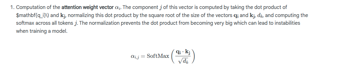
Note that dk is the size of the query and key vectors.

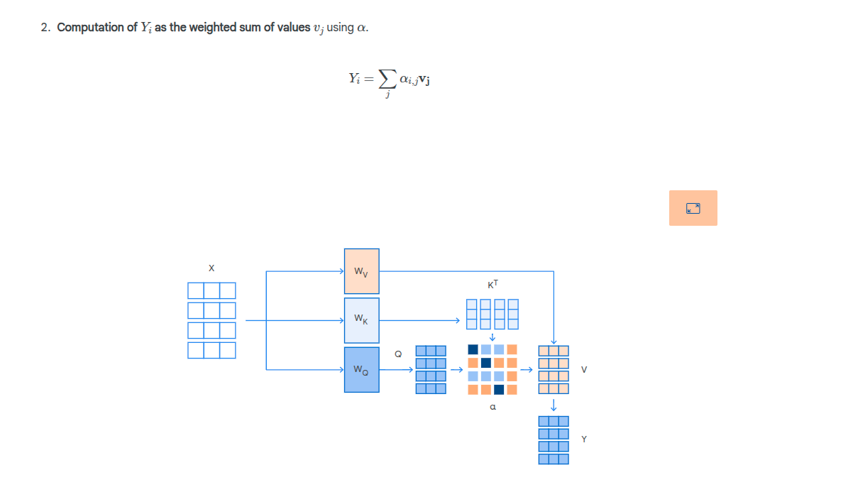
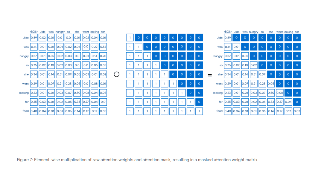
Masked Attention

Attention can be highly parallelized

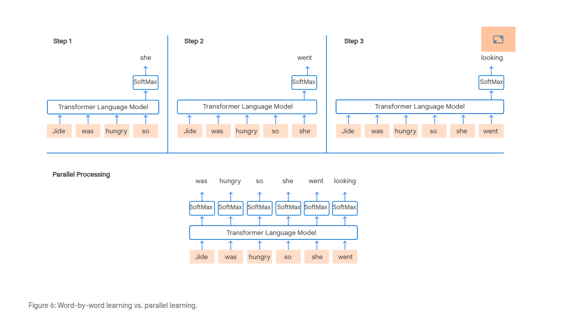
We don't want the model to be able to learn from future words if we're doing a parallel calculation. Therefore we want to mask off the future values, or set the weight to 0. We can do this by creating an attention mask.

Multi-Head Attention

These are paralell attention heads which allow us to capture different levels of dependencies in the text.

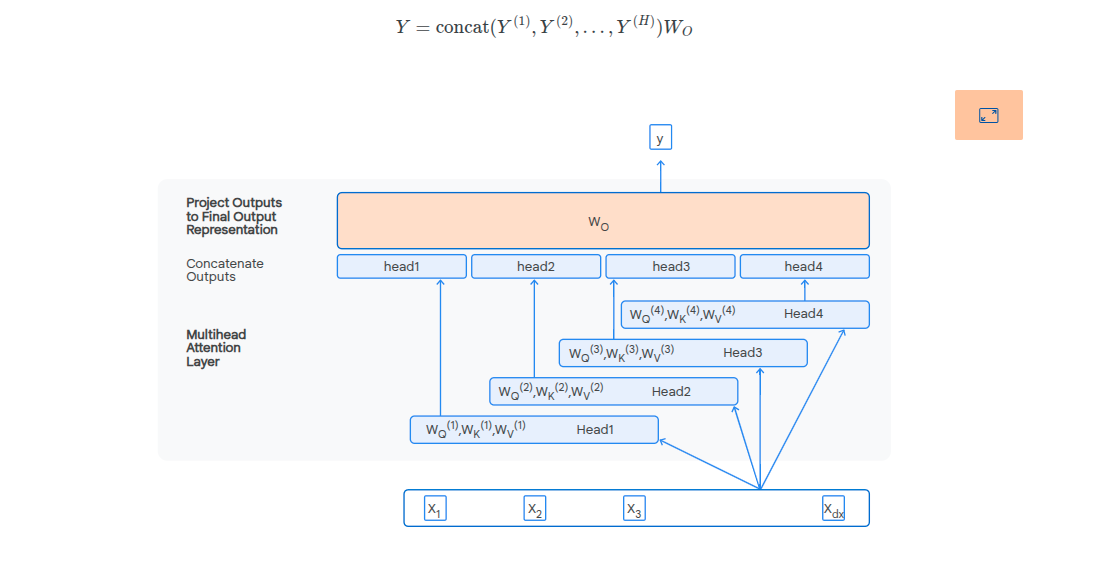
Syntactic dependencies

Dependencies required to make a sentence grammatically correct.

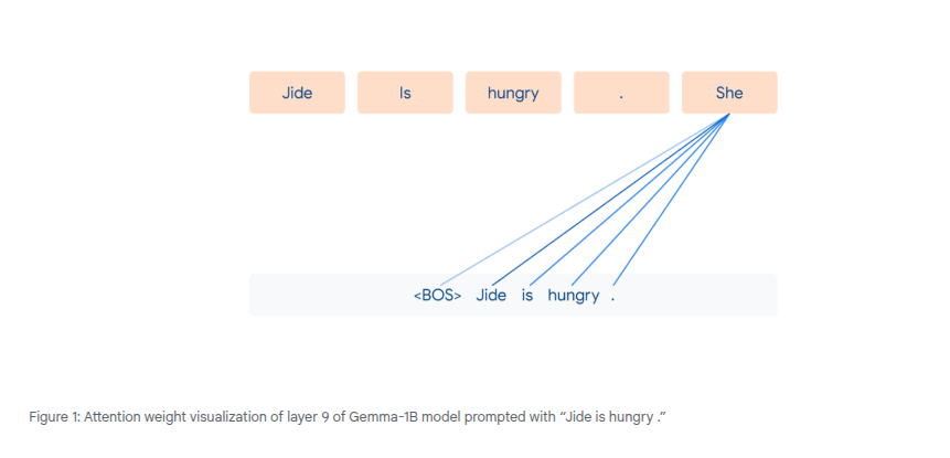
Co-reference dependencies

Multi word dependencies referring to the same subject e.g. "he", "she" refers to an entity previously references.

Coherence dependencies

Dependencies for making a text coherent.

To summarize, the attention mechanism is an effective method enabling
models to selectively and dynamically prioritize various segments of the
input sequence during the processing of every token. Its operation is
fundamentally structured around three components: queries (Q), keys (K),
and values (V). These are utilized to calculate relevance via dot
products, transform those scores into weights using the SoftMax function,
and finally generate a new token representation through a weighted sum of
the values.

Sinusoidal and Rotary Positional Embeddings

Because the attention mechanism is order invariant, positional information gets added using sinusoidal positional embeddings and rotary positional embeddings (RoPE).

Sinusoidal Embeddings

The input embedding at i has it's j'th component positional embedding calculated using sine or cosine based on whether the j'th component is odd or even:

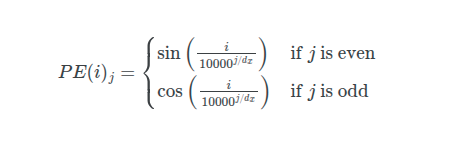
dx is the dimensions of the input embeddings.

The final input embedding which now contains the positional information is then calculated as:

This final position adjusted embedding is then used as the input to the first transformer block i.e. we've adjusted the input embeddings for positional information.

Rotary Positional Embeddings

Modifies the attention mechanism instead of the inputs.

THe query and key vectors are rotated according to their position to capture relative distance between tokens.

We see now that the dot product is that of the rotation of the query and key matrices. The theta represents a hyper-parameter of the model.

Transformer Blocks

There are 4 sub components in a transformer block, processing the input one after another:

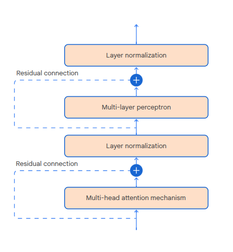
• Multi-head attention mechanism
• Layer normalization - used to stabilize model output
• MLP - introduces non-linearity required to learn complex patterns

The residual connections allow us to add the input from a component to it's output. Used for training convergence (prevent or detect when gradients get too small)?

Multi-layer Perceptron

Typically one layer with a non-linear activation function. Processes the output of the attention mechanism to produce the transformer block output.

The hidden layer has a higher dimensionality than the input layer, this is in order to allow the model to learn more complex feature representations in the hidden representation/layer before "compressing" to the lower dimensionality output.

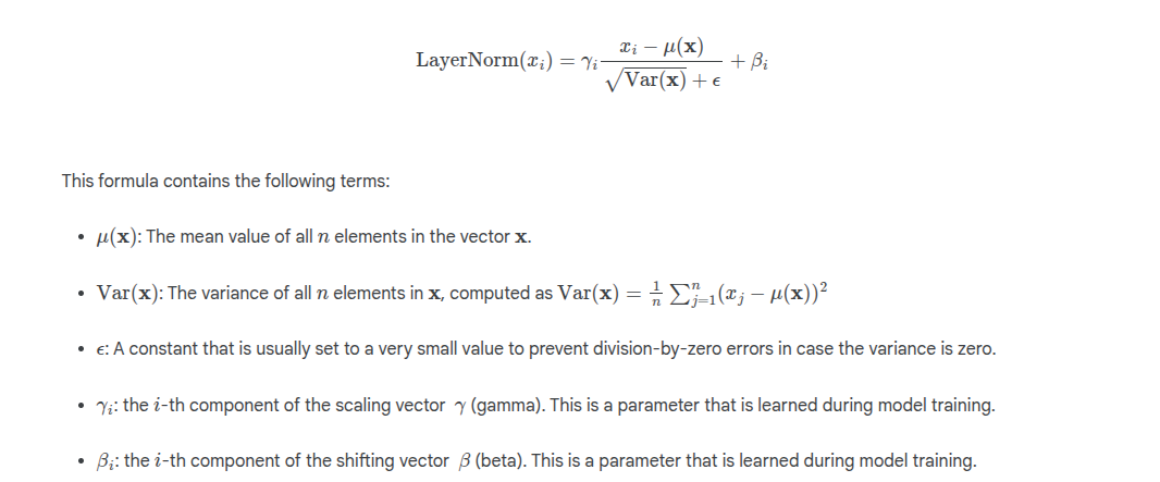
Layer Normalization

Used to ensure output values from a transformer block or the output values from the multi-head attention mechanism don't get too big or too small.

Very large or small output values result in large changes to gradients which results in unstable training.

Vanishing gradient problem - very small gradients, model weights not updated much

Exploding gradient problem - very large gradients, model weights changed drastically

The normalization calculation is a variant of Z-score with a scale and shift param:

Pros and Cons of Transformers

• High level of parallelism

• Good at modeling long range dependencies

• Attention mechanism is computationally quadratic - we have to compute the interaction between every token pair in the sequence so it's O(n^2)

• Computation+Memory intensive

• Require more training data than humans to aquire comparable skills

Humans are adept at extracting patterns and understanding from 
relatively sparse information, whereas transformers require 
extensive exposure to data to tune their parameters. 

Decoding and Generation

• Greedy decoding - chose the token with the highest probability. Continue until max number of tokens is generated, or an EOS is generated. Deterministically chooses the next token.

• Probabilistic sampling - generate the output token distribution. Select from this distribution using random sampling. Low probability tokens are still sometimes included in the sample output.

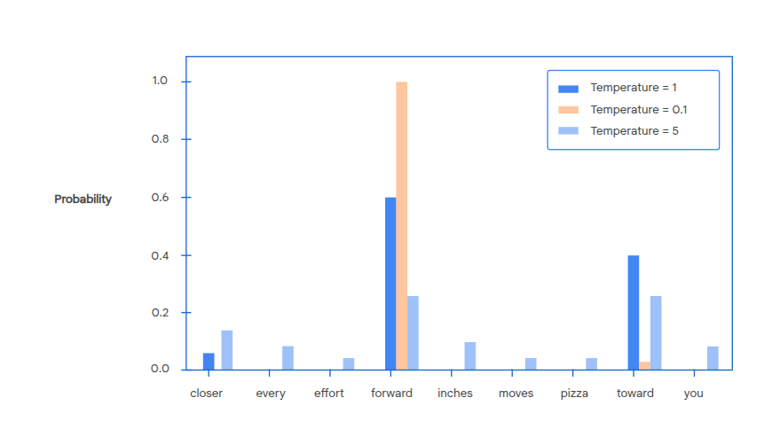
• Temperature based sampling - a parameter added to the SoftMax of the output layer.

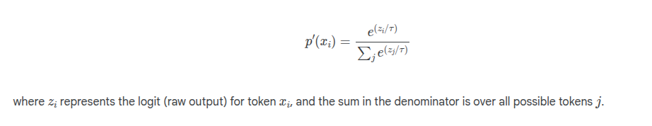
The temperature is used to create a modified output probability distro. A high temperature makes the distro more uniform (t > 1) whereas a low temperature concentrates on the most probably tokens (t < 1)

Top K Sampling

This approach ensures that the model focuses on the most likely options while still allowing for some degree of randomness and variation in the generated text.

We select the most probable k results, then re-normalise. Post re-normalization, we randomly sample from this reduced set.

Can be combined with temperature based sampling - you adjust the probability distribution based on temperature, then apply top k sampling.

Links and Resources

The Deep Learning Book

Evaluate model and system for safety